Economic Order Quantity (EOQ), Explained

Economic order quantity, EOQ, is a formula for finding the order size that minimizes your total inventory cost, balancing what it costs to place an order against what it costs to hold inventory on the shelf. It answers a narrower question than a reorder point does: a reorder point tells you when to order, EOQ tells you how much to order once you’ve decided to. The two work together, and most small distributors have heard of one and not the other.

The formula

EOQ = the square root of (2 x annual demand x cost per order, divided by annual holding cost per unit)

Three inputs go into it:

• Annual demand (D): how many units you sell in a year for that SKU.
• Order cost (S): what it costs to place a single order, shipping fees, receiving labor, any admin overhead tied to processing that PO.
• Holding cost (H): what it costs to keep one unit in stock for a year, warehouse space, insurance, capital tied up, and the risk of the item going stale or damaged while it sits.

A worked example. Say you sell 6,000 units a year of a SKU, it costs $50 to place and process each order, and it costs $4 per unit per year to hold it in stock. EOQ = the square root of (2 x 6,000 x 50 / 4), which works out to the square root of 150,000, or roughly 387 units per order. Order much less than that and you’re placing orders too often, paying the $50 order cost more times than you need to. Order much more and you’re tying up cash and shelf space holding inventory you won’t sell for months.

What EOQ is actually trading off

The logic behind the formula is straightforward once you see the two costs pulling in opposite directions. Order in small batches frequently, and your holding cost drops (less inventory sitting around at any given moment) but your ordering cost climbs (more orders, more shipping fees, more receiving labor). Order in large batches rarely, and it flips: ordering cost drops, holding cost climbs. EOQ finds the order size where those two costs are balanced, and the total is lowest.

That’s genuinely useful math. A reorder point tells you the trigger, the stock level where a new order needs to go out. EOQ tells you the size of that order once triggered. Used together, they answer both halves of a purchasing decision that a lot of small teams still answer by gut feel, ordering “about what we usually order” without ever checking whether that number is actually efficient.

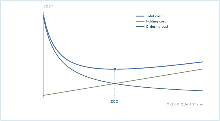
Holding cost rises with order size, ordering cost falls, and the total cost curve bottoms out at the EOQ.

Where the formula breaks down

EOQ was built on an assumption that doesn’t hold for most real inventory: constant, steady demand. The formula treats annual demand as a single fixed number, divided evenly across the year. A SKU that sells 500 units a month, every month, fits that assumption reasonably well. A SKU with a strong holiday spike, a seasonal product, or anything whose demand swings with promotions or the calendar doesn’t.

Run the formula on a SKU with real seasonality and you get one order size calculated off an annual average, applied the same way in a slow month and a peak month. Order that fixed amount in October ahead of a December spike, and you’re short. Order the same fixed amount in February after the spike’s passed, and you’re sitting on dead stock that won’t move again until next year’s season. The formula also assumes order costs and holding costs are stable numbers you actually know, which is a reasonable estimate for a stable operation but gets shakier the more supplier pricing or shipping costs move around.

None of this makes EOQ useless, it’s a solid starting point for a stable, low-variance SKU, and a useful way to sanity-check whether your current order sizes are wildly inefficient. It’s a poor fit as the only method for anything with real demand variability, which describes a meaningful share of most distributors’ catalogs.

What a dynamic approach looks like instead

The gap EOQ leaves is exactly what demand forecasting is built to close: instead of one static annual-average number, forecasting demand without a data team means looking at actual sales history, seasonality, and current supplier lead times together, so the recommended order size for a SKU in November reflects November’s expected demand, not a number averaged across a year that includes both a slow February and a busy December. That same forecast also feeds safety stock, the buffer that covers demand or lead time uncertainty EOQ’s clean formula doesn’t account for at all.

A practical way to use both

If you’re not currently running any formal order-sizing math, calculating EOQ for your highest-volume, most stable SKUs is a reasonable place to start, it’s a five-minute calculation and it’ll likely reveal at least one or two SKUs where your current order size is costing more than it needs to in either shipping frequency or holding cost. For anything seasonal, promotional, or genuinely variable, treat the EOQ number as a floor or a sanity check rather than the answer, and lean on a forecast that actually accounts for how that SKU’s demand moves through the year.

What Flowbound does and doesn’t do here

Flowbound doesn’t run a static EOQ calculation and hand you one fixed number to reorder forever. What Reorder does is place the purchase order the moment your reorder point is hit, at a quantity already recommended from your actual sales history, seasonality, and current supplier lead times, the same inputs Demand Forecasting uses, so the order size adapts to what’s actually happening with that SKU instead of an annual average calculated once and never revisited. Confidence thresholds still govern which of those orders go out automatically and which get flagged for a second look, so the system doesn’t blindly trust its own math any more than you’d blindly trust a static formula.

FAQ

What is economic order quantity (EOQ)? EOQ is a formula that calculates the order size that minimizes total inventory cost, balancing the cost of placing an order against the cost of holding inventory. The formula is the square root of (2 x annual demand x order cost, divided by annual holding cost per unit).

How is EOQ different from a reorder point? A reorder point answers when to place an order, the stock level that triggers a purchase. EOQ answers how much to order once that trigger fires. They’re complementary calculations, not competing ones.

Does EOQ work for seasonal products? Not well. EOQ assumes constant demand spread evenly across the year, so a SKU with real seasonal swings gets one fixed order size calculated off an annual average, too small ahead of a peak and too large right after one. Demand forecasting that accounts for seasonality directly is a better fit for those SKUs.

Is EOQ still worth calculating for a small distributor? Yes, for stable, steady-demand SKUs it’s a quick way to check whether your current order sizes are efficient. For anything with real demand variability, treat it as a starting point or a sanity check rather than the final answer.

What replaces EOQ for products with unpredictable demand? A forecast-driven approach that recalculates recommended order size as sales history, seasonality, and safety stock needs change, rather than relying on one static number calculated once a year.